seq2seq 모델은 고정된 크기의 벡터로 압축하는 과정에서 정보가 손실되고, RNN의 고질적 문제인 기울기 소실 문제가 존재한다. 이로 인해 입력 시퀀스가 길어질수록 출력 시퀀스의 정확도가 떨어진다. 이를 보정하기 위한 attention 기법을 알아보자.
# 15-01 Attention Mechanism
1. Attention이란?
디코더에서 출력 단어를 예측하는 매 시점마다 인코더의 전체 입력 문장을 다시 참고하는 것.
이 때, 전체 입력 문장 중에서도 해당 시점에서 예측할 단어와 관련된 입력 단어에 더 집중(attention)한다.
여러 종류의 Attention이 있지만, Attention Score를 구하는 방법만 다르다.

'dot' attention은 루옹 어텐션이라고도 하며, 'concat' attention은 바다나우 어텐션이라고도 한다.
2. Attention Function
Attention(Q, K, V) = Attention Value
어텐션 함수는 주어진 Q(Query)에 대한 모든 K(Key)와의 유사도를 구한다.
각 유사도는 K와 매핑되어있는 각 V(Value)에 반영한다.
유사도가 반영된 V들을 모두 더해 리턴한 것이 바로 어텐션 값(Attention Value)
Q = Query : t 시점의 디코더 셀에서의 은닉 상태
K = Keys : 모든 시점의 인코더 셀의 은닉 상태들
V = Values : 모든 시점의 인코더 셀의 은닉 상태들
3. Dot-Product Attention(루옹 어텐션)
다양한 Attention 종류 중에서 가장 이해하기 쉬운 Dot-Product Attention을 먼저 공부한다.
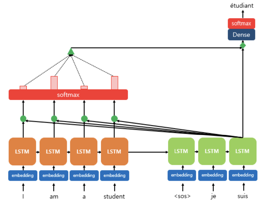
위 그림에서, 디코더(초록색)의 각 LSTM 셀은 출력단어를 예측하기 위해 인코더의 모든 입력단어 정보를 다시 참고한다.
참고할 입력단어들은 소프트맥스 함수를 거친 각 단어의 결과값들의 묶음(초록 삼각형)이다.
구체적으로 단계를 살펴보자.
(1) Attention Score 구하기
Attention Score = t시점에서 디코더의 은닉상태 s가 인코더의 모든 은닉상태 h와 각각 얼마나 유사한지 판단하는 스코어값으로, s를 전치하고 각 h와 내적을 수행한 스칼라값임

Attention Score들의 묶음을 e라고 한다.

(2) Attention Distribution 구하기
Attention Distribution = e에 소프트맥스를 적용해 얻은 확률 분포
Attention Weight = 어텐션 분포 속 각각의 값

Attention Distribution을 알파라고 한다.

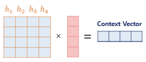
(3) Attention Value(=Context vector) 구하기
Attention Value = 인코더의 각 은닉상태 h와 각 어텐션 가중치값들을 곱하고 모두 더한 가중합

최종 Attenton Value를 a라고 한며, context vector라고도 한다.

(4) Attention Value와 디코더의 은닉상태 s를 연결
최종 어텐션 값 a와 디코더의 은닉상태 s를 결합(concatenate)하여 하나의 벡터 v로 만든다.

(5) 출력층으로 갈 최종 입력값 연산
최종적으로 신경망 연산을 한 번 더 추가한다. v에 가중치행렬을 곱하고 tanh 함수를 지나게 한다.

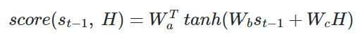
4. Bahdanau Attention(바다나우 어텐션)
Attention(Q, K, V) = Attention Value 에서 Query가 t-1 시점의 디코더의 은닉상태라는 점이 다름. 즉, Attention score를 구할 때 st 대신 st-1 사용
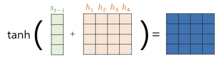
(1) Attention score 구하기


그 이후의 작업은 똑같다. 어텐션 분포 -> 어텐션 값 -> 최종 입력값
(2) Attention Distribution 구하기

(3) Attention Value(=Context vector) 구하기
(4) Attention Value와 디코더의 은닉상태 st-1를 연결
(5) 출력층으로 갈 최종 입력값 연산

마지막으로 최종 입력값 st는 출력층으로 전달되고, t시점의 예측값 y를 구한다.
# 15-02 Attention으로 리뷰 감성분류 실습
텍스트분류에서 어텐션 메커니즘을 사용하는 이유: RNN이 time step을 지나며 손실했던 정보들을 다시 참고하기 위해
1. Bahdanau Attention
데이터 전처리는 마쳤다는 가정 하에 코드를 이어간다.
import tensorflow as tf

class BahdanauAttention(tf.keras.Model):
  def __init__(self, units):
    super(BahdanauAttention, self).__init__()
    self.W1 = Dense(units)
    self.W2 = Dense(units)
    self.V = Dense(1)

  def call(self, values, query): # 단, key와 value는 같음
    # query shape == (batch_size, hidden size)
    # hidden_with_time_axis shape == (batch_size, 1, hidden size)
    # score 계산을 위해 뒤에서 할 덧셈을 위해서 차원을 변경해줍니다.
    hidden_with_time_axis = tf.expand_dims(query, 1)

    # score shape == (batch_size, max_length, 1)
    # we get 1 at the last axis because we are applying score to self.V
    # the shape of the tensor before applying self.V is (batch_size, max_length, units)
    score = self.V(tf.nn.tanh(
        self.W1(values) + self.W2(hidden_with_time_axis)))

    # attention_weights shape == (batch_size, max_length, 1)
    attention_weights = tf.nn.softmax(score, axis=1)

    # context_vector shape after sum == (batch_size, hidden_size)
    context_vector = attention_weights * values
    context_vector = tf.reduce_sum(context_vector, axis=1)

    return context_vector, attention_weights
2. BiLSTM+Attention
from tensorflow.keras.layers import Dense, Embedding, Bidirectional, LSTM, Concatenate, Dropout
from tensorflow.keras import Input, Model
from tensorflow.keras import optimizers
import os

# 모델 설계
# 입력층 설계
sequence_input = Input(shape=(max_len,), dtype='int32')
# 임베딩층 설계
embedded_sequences = Embedding(vocab_size, 128, input_length=max_len, mask_zero = True)(sequence_input)
# BiLSTM 의 첫번째층 설계
lstm = Bidirectional(LSTM(64, dropout=0.5, return_sequences = True))(embedded_sequences)
# BiLSTM 의 두번째층 설계
lstm, forward_h, forward_c, backward_h, backward_c = Bidirectional \
  (LSTM(64, dropout=0.5, return_sequences=True, return_state=True))(lstm)
# 순방향과 역방향의 은닉상태와 셀상태를 연결
state_h = Concatenate()([forward_h, backward_h]) # 은닉 상태
state_c = Concatenate()([forward_c, backward_c]) # 셀 상태
# 어텐션 값, 어텐션 가중치 계산
attention = BahdanauAttention(64) # 가중치 크기 정의
context_vector, attention_weights = attention(lstm, state_h)
# 출력층 설계
dense1 = Dense(20, activation="relu")(context_vector)
dropout = Dropout(0.5)(dense1)
output = Dense(1, activation="sigmoid")(dropout)
model = Model(inputs=sequence_input, outputs=output)
model.compile(loss='binary_crossentropy', optimizer='adam', metrics=['accuracy'])
# 모델 훈련
history = model.fit(X_train, y_train, epochs = 3, batch_size = 256, validation_data=(X_test, y_test), verbose=1)# 테스트 데이터에 대해 모델 평가
print(model.evaluate(X_test, y_test)[1]) # 0.8793
'딥러닝 > 딥러닝을 이용한 자연어처리 입문' 카테고리의 다른 글
| [딥러닝 NLP] 17. BERT(MLM, NSP), SBERT (0) | 2024.02.18 |
|---|---|
| [딥러닝 NLP] 16. Transformer (1) | 2024.02.07 |
| [딥러닝 NLP] 14. RNN encoder-decoder (1) | 2024.02.06 |
| [딥러닝 NLP] 13. Subword Tokenizer(BPE, SentencePiece, Huggingface) (0) | 2024.02.01 |
| [딥러닝 NLP] 12. Tagging Task 실습(NER, POS) (1) | 2024.02.01 |


